WiscKey: Separating Keys from Values in SSD-Conscious Storage

Posted on March 10, 2023  •  27 minutes  • 5725 words

LSM-tree (Log structured merge tree) is a data structure typically used for write-heavy workloads. LSM-tree optimizes the write path by performing sequential writes to disk. WiscKey is a persistent LSM-tree-based key-value store that separates keys from values to minimize read and write amplification. The design of WiscKey is highly SSD optimized, leveraging both the device’s sequential and random performance characteristics.

This article summarises the WiscKey paper published in 2016.

Before we understand the paper, it is essential to understand the LSM-tree data structure, read and write amplification in the LSM-tree and various SSD characteristics that should be considered while building an SSD-conscious storage engine.

LSM-tree

LSM-tree is a write-optimized data structure implemented by storage engines for supporting write-heavy workloads. A lot of storage engines including BadgerDB , RocksDB and LevelDB use LSM-tree as the core data structure.

Storage engine is a software module that provides data structures for efficient reads and writes. The two most common data structures are B+Tree (read-optimized) and LSM-tree (write-optimized).

Let’s look at the structure of LSM-tree to understand why it is write-optimized.

LSM-tree buffers the data in memory and performs a sequential write to disk after the in-memory buffer is full. The image below highlights the throughput difference between sequential and random writes on an NVMe SSD; the difference would be much higher on an HDD.

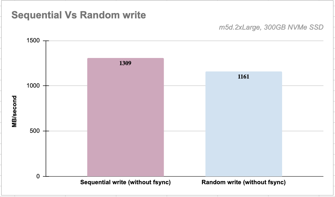
LSM-tree-based storage engines offer better write throughput by performing sequential writes to disk.

LSM-tree consists of components of exponentially increasing sizes, C0 to Ck. C0 is a RAM resident component that stores key-value pairs sorted by key and supports efficient writes and reads, whereas C1 to Ck are immutable disk-resident components sorted by key.

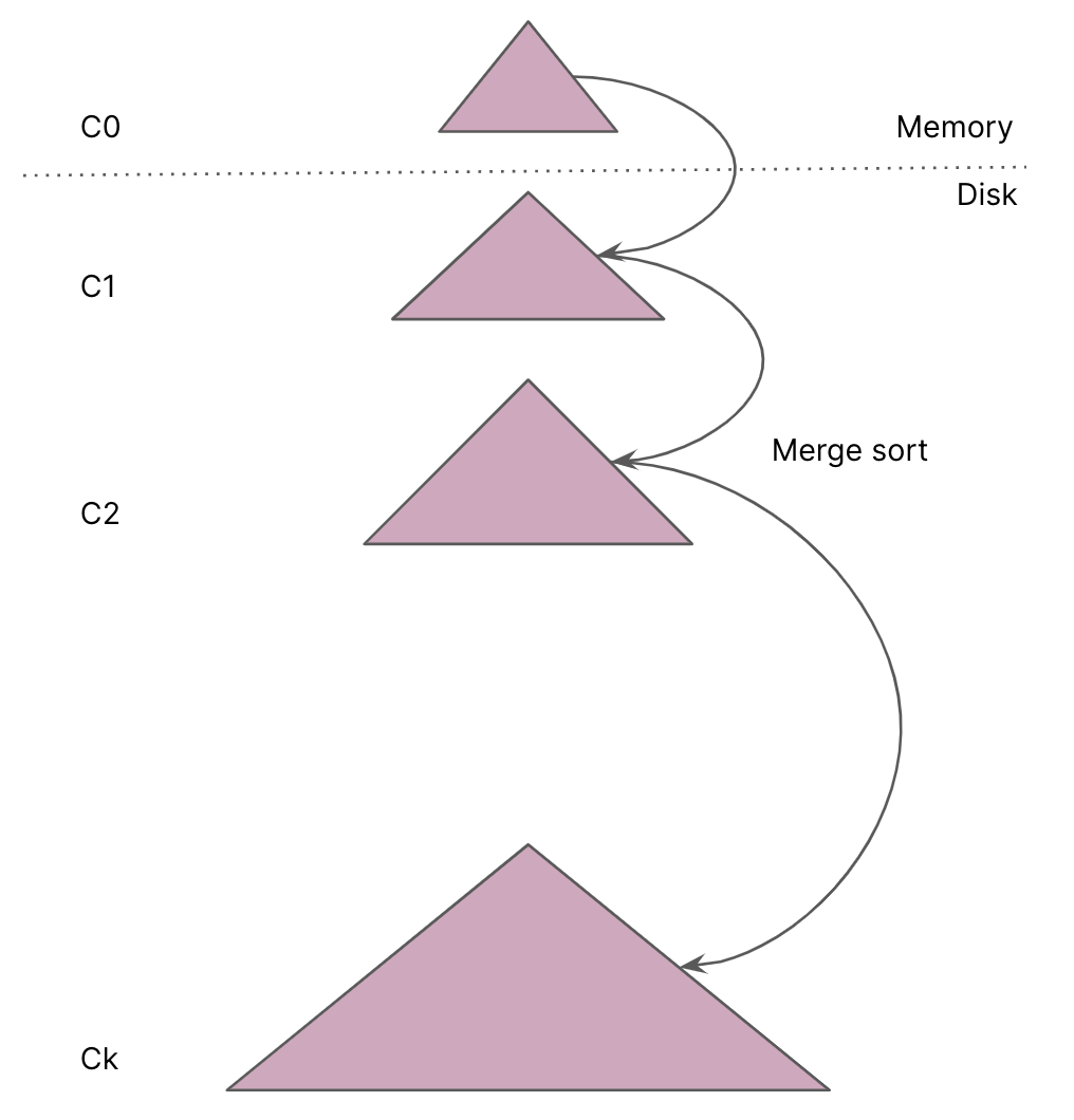
Data structure choice for C0: The data structure for C0 should maintain the keys in the sorted order (for range queries) and provide efficient reads and writes. This data structure could be a hashmap , a treemap or a red-black tree or a skip list . Of all these data structures, the Skip list is the one that supports versioned keys, the same key with different versions.

Let’s take a look at the overall flow of put(key: []byte, value: []byte) and get(key: []byte) operations in the LSM-tree.

Every put(key, value) in the LSM-tree adds the key-value pair in the C0 component, and after C0 is full, the entire data is flushed to disk. LSM-trees treat delete(key) as another put, which will put the key with a deleted marker.

After C0 is full, a new instance of C0 is created and the entire in-memory data is flushed to disk. All in-memory data consisting of key-value pairs is encoded in a byte array and written to disk. If the C1 component already exists on disk, the buffered content is merged with the contents of C1.

Because all the new writes are kept in-memory, they can get lost in case of a failure. The durability guarantee is ensured by using a WAL . Every put(key, value) appends the key-value pair to a WAL file and then writes the key-value pair to the C0 component. Appending to a WAL file is also a sequential write to disk.

Every get(key) in the LSM-tree goes through the RAM based component to disk components from C1 to Ck in the order. The get(key) operation first queries the C0 component, if the value for the key is not found, the search proceeds to the disk resident component C1. This process continues until the value is found or all the disk resident components have been scanned. LSM-trees may need multiple reads for a point lookup. Hence, LSM-trees are most useful when inserts are more common than lookups.

Quick summary

LSM-tree is a collection of exponentially increasing sized components, C0 to Ck.
Writes go to WAL (on disk) -> C0 (in RAM).
After C0 is full, the entire data is flushed to disk.
The get operation involves going through C0 to Ck.

Let’s look at the structure of LSM-tree in LevelDB to understand more on C0 to Ck components.

LevelDB

LevelDB is a key-value storage engine based on LSM-tree. LevelDB maintains the following data structures:

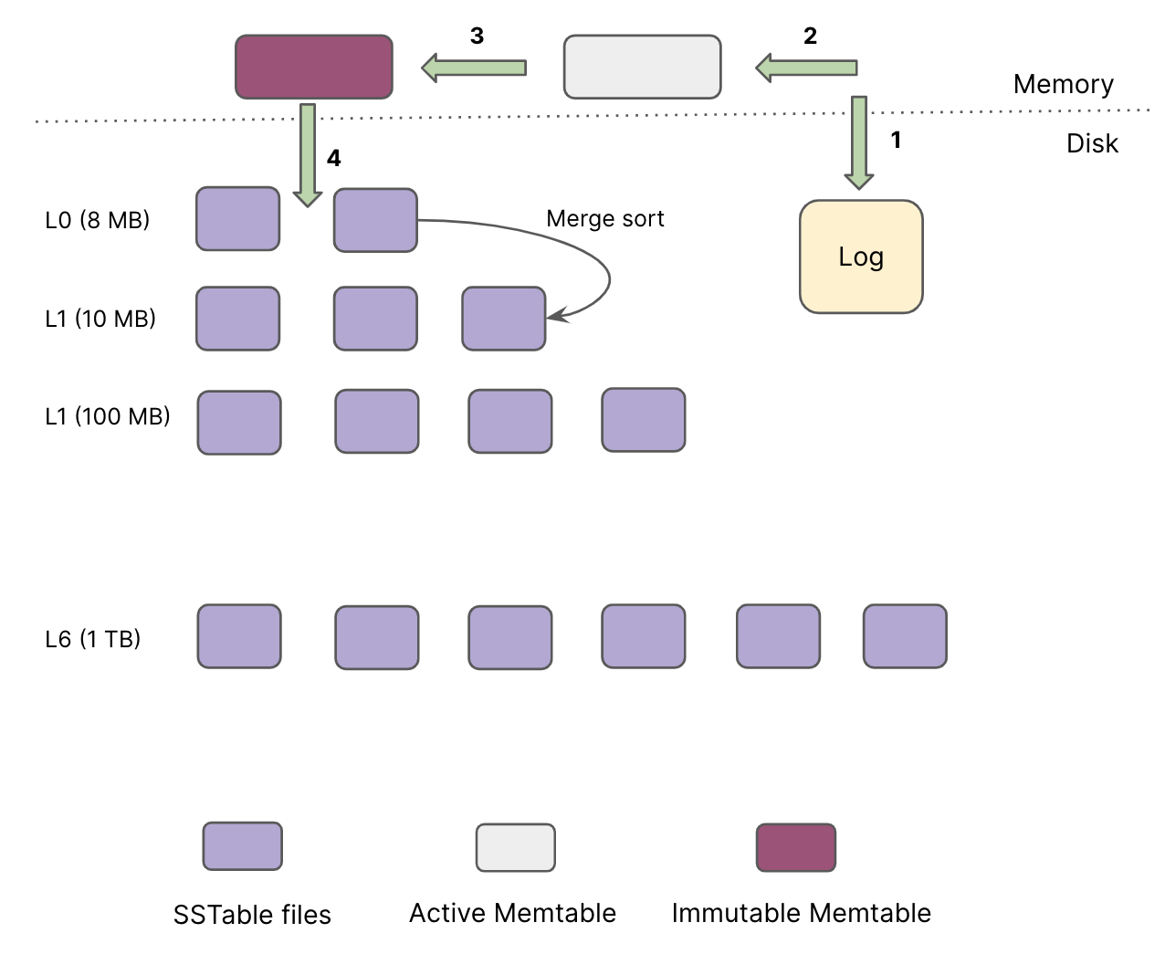
1. On-disk log file (WAL) to persist the writes
2. Two in-memory components called “memtables” (active and passive)
3. Seven levels of on-disk components called “SSTable” (Sorted string table)

Every put(key, value) goes in a log file and the active in-memory memtable. Once the active memtable is full, LevelDB switches to a new memtable and log file to handle further writes.

The previously active memtable is stored as an immutable memtable in RAM and flushed to disk in the background. This flush to disk generates a new SSTable file (about 2 MB) at level-0 and discards the previous log file (WAL).

The size of all files in each level is limited and increases by a factor of ten with the level number. For example, the size limit of all files at L1 is 10 MB, while the limit of L2 is 100 MB.

In order to perform the get(key) operation, LevelDB performs the following steps:

1. Perform get in the active memtable (RAM),
2. If not found, perform get in the immutable memtable (RAM),
3. If not found, perform get in the files from Level0 to Level6. LevelDB ensures that the keys do not overlap in the files from Level1 to Level6 whereas keys in the Level0 files can overlap.
   1. This means that a get operation may involve multiple files in Level0 and one file at each level from Level1 to Level6

LevelDB implements the in-memory components using Skip list .

LevelDB stores keys in the memtable with versions (or tags). It is possible to insert the key “Storage” more than once; each time, it will have a different version. Such storage engines are called versioned storage engines. Skip list is a natural data structure choice for building versioned stores because it will place the same key with different versions next to each other. Below is the definition of Add method in LevelDB’s memtable. The key-value pair and sequence number (u64) are encoded together.

void MemTable::Add(SequenceNumber s, ValueType type, const Slice& key,
                   const Slice& value) {
  // Format of an entry is concatenation of:
  //  key_size     : varint32 of internal_key.size()
  //  key bytes    : char[internal_key.size()]
  //  tag          : uint64((sequence << 8) | type)
  //  value_size   : varint32 of value.size()
  //  value bytes  : char[value.size()]
  size_t key_size = key.size();
  size_t val_size = value.size();
  size_t internal_key_size = key_size + 8;
  const size_t encoded_len = VarintLength(internal_key_size) +
                             internal_key_size + VarintLength(val_size) +
                             val_size;
  char* buf = arena_.Allocate(encoded_len);
  char* p = EncodeVarint32(buf, internal_key_size);
  std::memcpy(p, key.data(), key_size);
  p += key_size;
  EncodeFixed64(p, (s << 8) | type);
  p += 8;
  p = EncodeVarint32(p, val_size);
  std::memcpy(p, value.data(), val_size);
  assert(p + val_size == buf + encoded_len);
  table_.Insert(buf);
}

Let’s understand the high-level architecture of LevelDB.

Let’s spend a few minutes understanding an SSTable file’s structure before we move on.

SSTables contain key-value pairs sorted by key. Key-value pairs are encoded before they can be written to a file. One encoding scheme could be to use key-size, followed by value-size, followed by the actual key and then the actual value as depicted in the following table:

We use u32 type as an example for the key and the value size. Key-size and value-size would be represented using fixed-size data types like u16 or u32.

A naive way to get the value for a key in an SSTable would be to read the entire SSTable file, match each key and return the value if the matching key is found.

How do you read a single key-value pair from an SSTable file that follows the encoding mentioned above scheme? To read one key-value pair from an SSTable file, we need to read the first four bytes (u32) to get the key size, next four bytes to get the value size, then read the number of bytes equal to the key size to get the key and finally read the number of bytes equal to the value size to get the value.

SSTable files are organized into blocks (or sections). SSTable files in all the LSM-tree based storage engines typically include index-block + bloom-filter-block + data-block. Imagine all these blocks as byte arrays ranging from offset to offset.

Index-block contains the key-offset pairs in the sorted order by key. The offset here is the offset of the key-value pair in the data block of the SSTable file.

Bloom filter block contains the bloom filter byte array of all the keys present in the SSTable file

Data block contains the actual data; the key-value pairs in the sorted order by key

A Bloom filter is a probabilistic data structure used to test whether an element is a set member. A bloom filter can query against large amounts of data and return either “possibly in the set” or “definitely not in the set”. More information on bloom filter is available here .

Let’s take a quick look at compaction.

Compaction

To maintain the size limit of each level, once the total size of a level L_i exceeds its limit, the compaction thread will choose one file from L_i, merge sort with all the overlapped files of L_i+1, and generate new L_i+1 SSTable files. The compaction process involves:

• Loading SSTable files in memory,
• Performing merge sort on the files,
• Removing the deleted keys and writing back those files. The compaction thread continues until all levels are within their size limits.

Compaction is a CPU & IO-intensive process and the reason for high write-amplification in LevelDB.

Quick summary

LevelDB uses WAL, memtables and SSTables as its data structures.
Memtable is implemented using Skip list
SSTables are sorted string tables and organized into levels, Level0 to Level6.
SSTables are organized into index-block, bloom-filter, and data blocks.
Puts go to WAL and the active memtable.
Gets go to active memtable -> immutable memtable -> SSTables.

Let’s now understand “read and write amplification”.

Read Write amplification

HDDs, SDDs and NVMe SSDs are block storage devices. The smallest unit of exchange between an application and a block storage device is a block. Usually the size of a block is 4KB. Let’s assume a key/value storage engine on a block storage device like HDD. When the key/value storage engine wants to fetch the value for a 128 bytes key, it must do the following:

• read the entire block containing the value from the underlying device (ignore how that block is located),
• allocate a buffer in-memory to hold the result

Even when making a minor update say, 128 bytes, the storage engine needs to do the following:

• read the entire block containing those 128 bytes into a memory buffer,
• update 128 bytes in the buffer,
• write the entire block to the underlying device.

Block IO involves transferring an entire block of data, typically 4K bytes at a time. So the task to read 128 bytes would require reading at least one block of 4K bytes.

The storage engine has to read (and write to) more than what is requested by the user. This results in “amplification”. Both the reads and the writes get amplified.

Read amplification is the ratio of the amount of data read from the storage device and the amount of data requested by the user. In the above example, read amplification is 32 (4*1024 bytes / 128 bytes).

Write amplification is the ratio of the amount of data written to the storage device and the amount of data requested by the user. In the above example, write amplification is 32 (4*1024 bytes / 128 bytes).

Quick summary

The smallest unit of data exchange between an application and a block storage device is a block, usually 4KB in size.
Read/Write amplification is the amount of data read from (or written to) the storage device and the amount of data requested by the user.

Analysis of Read Write amplification in LevelDB

Let’s analyze the read-and-write amplification in LevelDB.

Let’s start with read amplification.

LevelDB ensures that the keys do not overlap in the files from Level1 to Level6 whereas keys in the Level0 files can overlap.

Let’s assume that the value for a key is not found in the active and the immutable memtable. Now, LevelDB needs to read SSTable files. In the worst case, LevelDB needs to check eight files in Level0, and one file for each of the remaining six levels: a total of 14 files.

To find the value for a key within an SSTable file, LevelDB needs to read multiple metadata (or index) sections within the file. Specifically, the amount of data read is: 16-KB index section, a 4-KB bloom-filter section, and a 4-KB data section (24KB).

The read amplification in LevelDB is 336 (14 files * 24KB). Another way to state this is: “LevelDB amplifies the reads by 336 times in the worst case”.

Let’s analyze the write amplification.

LSM-tree based storage engines must perform file merges during compaction .

In LevelDB, the size of the level L_i is ten times the size of the level L_i-1 (Size of Level2 is 100MB whereas the size of Level1 is 10MB). To merge a file from the level L_i-1 to L_i, LevelDB may end up reading ten files from the level L_i in the worst case and write back those ten files after sorting. So, the write amplification of moving a file from one level to the next can be as high as ten.

In the worst case, a file may move from Level0 to Level6 through compaction steps. The total write amplification in the worst case can be over 50 (write amplification is 10 for each level between L1 to L6).

We ignore the cost of moving a file from Level0 to Level1.

Why does LevelDB check only one SSTable file at each level from Level1 to Level6, for a read operation?

LevelDB ensures that the keys do not overlap in the files from Level1 to Level6. This means a range-based search on keys can be done in RAM to identify an SSTable at each level to search.

This approach can be highlighted with the following pseudocode:

    //Compare the incoming key against the biggest keys in all the SSTable files at each level. 
    //BiggestKey can be maintained in RAM for each SSTable file from level >= 1.
	idx := sort.Search(len(level.table_files), func(index int) bool {
		return CompareKeys(level.table_files[index].BiggestKey(), key) >= 0 
	})
	if idx >= len(level.table_files) {
		// Given key is strictly > than every element we have.
		return nil
	}
	return level.table_files[idx]

Hence, LevelDB has to search one SSTable file at each level from Level1 to Level6 in the worst case.

Why is the size of the index section 16KB?

SSTables can contain more than one metadata or index section. Even if the index section is just 1KB, Block IO involves reading the entire disk block from the underlying storage. LevelDB has four index sections; each section involves reading a 4KB disk block. Hence, the data that is actually read for the index section is 16KB.

Why is the size of the data section just 4KB?

The data section can be huge, but LevelDB needs to read just the 4KB data section to find the value for a key. The steps include:

• LevelDB will load the index section to identify the position of the bloom-filter section.
  • Index section (or the index block) contains metadata, and one of the metadata items could be the beginning offset of the bloom-filter block (the other could be the offset of the keys in the data block as mentioned earlier).
• LevelDB will load the bloom-filter section and skip the file if the key is not present.
• If the bloom filter indicates that the key may be present, LevelDB will identify the offset of the key from the index section.
• LevelDB jumps to the identified offset within the data section. With Block IO, the entire block containing the offset is read. So, LevelDB ends up reading 4KB of the data block.

I am using the term section with index, bloom-filter and data to avoid confusing it with the disk block.

Why do we need an index block in an SSTable file?

In a key-value storage engine, the value is considered to be much bigger than the key.

Index block will contain the key/value-offset pairs sorted by keys. Let’s assume 10,000 keys in an SSTable file where each key is 100 bytes long. This means each key-offset pair will take 104 bytes (100 bytes for the key + 4 bytes for the offset, ignoring the encoding). So, the total size of the index block would be around 0.99 MB (((104 * 10,000)/1024)/1024). To get the value for a key, the storage engine will need to read ~1 MB of index block, and if the key is found, a random seek to the identified offset within the data block will be needed.

If the index block were not there, the same get operation would have happened against the data block. Assuming the size of a single value to be 1024 bytes, we will have around 10.71 MB ((((100 + 1024) * 10,000)/1024)/1024) as the size of the data block.

Quick summary

The read amplification in LevelDB is 336 and the write amplification can be over 50, in the worst case.
A key idea while designing a storage engine is to minimize the read and write amplification to reduce IO latency. Also, SSDs can wear out through repeated writes, and the high write amplification in LSM-trees can significantly reduce device lifetime.

SSD considerations when designing a storage engine

There are fundamental differences between SSDs and HDDs which should be considered when designing a storage engine. Let’s look at some of the most important considerations:

1. SSDs can wear out through repeated writes, the high write amplification in LSM-trees can significantly reduce the device lifetime.
2. SSDs offer a large degree of internal parallelism

Point 1 means we should try to reduce the write amplification when designing a storage engine for SSD-conscious storage. We have already seen that the compaction process is the source of high write-application in LSM-tree based storage engines.

Point 2 means we should try to leverage the parallelism offered by SSDs when performing IO operations. Let’s look at the below graph. For the request size >= 64KB, the aggregate throughput of random reads with 32 threads matches the sequential read throughput.

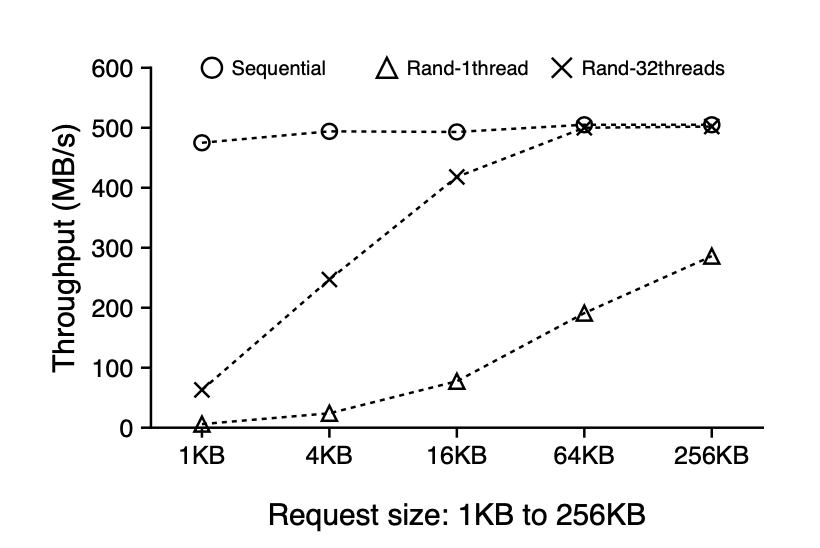
Sequential and Random Reads on SSD. This figure shows the sequential and random read performance for various request sizes on a modern SSD device. All requests are issued to a 100-GB file on ext4.

Quick summary

When designing a storage engine for SSDs, try to reduce the write-amplification and leverage the internal parallelism offered by SSDs.

With these considerations, let’s understand WiscKey proposal.

WiscKey proposal

WiscKey proposes four key ideas:

1. Separate values from keys, keeping only the keys in the LSM-tree, putting values in a separate value-log.
2. Leverage the parallel random read characteristic of SSDs during range queries.
3. Introduce garbage collection to remove values corresponding to deleted keys from value-log.
4. Remove LSM-tree log (WAL log) without sacrificing consistency (under Optimizations ).

Let’s discuss each of these ideas one by one.

Separate values from keys

Compaction is the reason for the significant performance cost in LSM-trees. Multiple SSTable files are read in-memory during compaction, sorted, and written back. This is also the reason for the high write amplification in LevelDB. If we look at the compaction process carefully, we will realize that this process only needs to sort the keys, while values can be managed separately. Since keys are usually smaller than values, compacting only keys could significantly reduce the amount of data needed during the sorting.

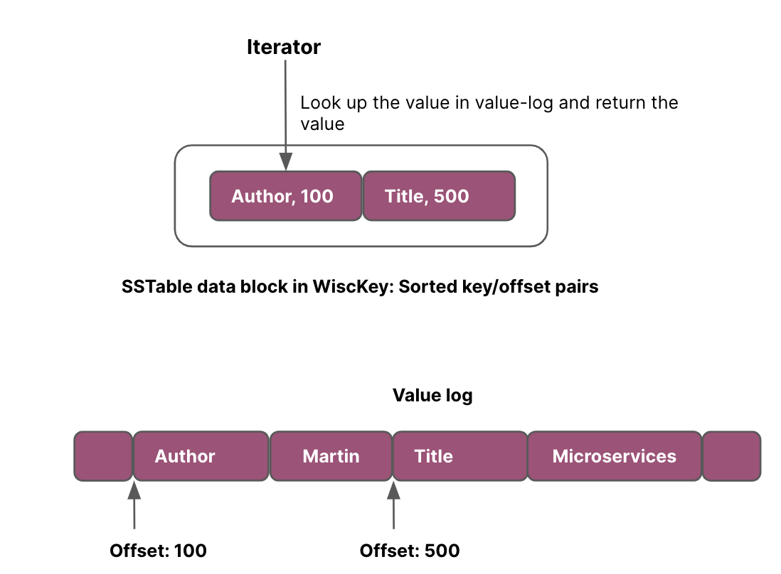
In WiscKey, only the location of the value is stored in the LSM-tree along with the key, while the actual values are stored in a separate value-log file.

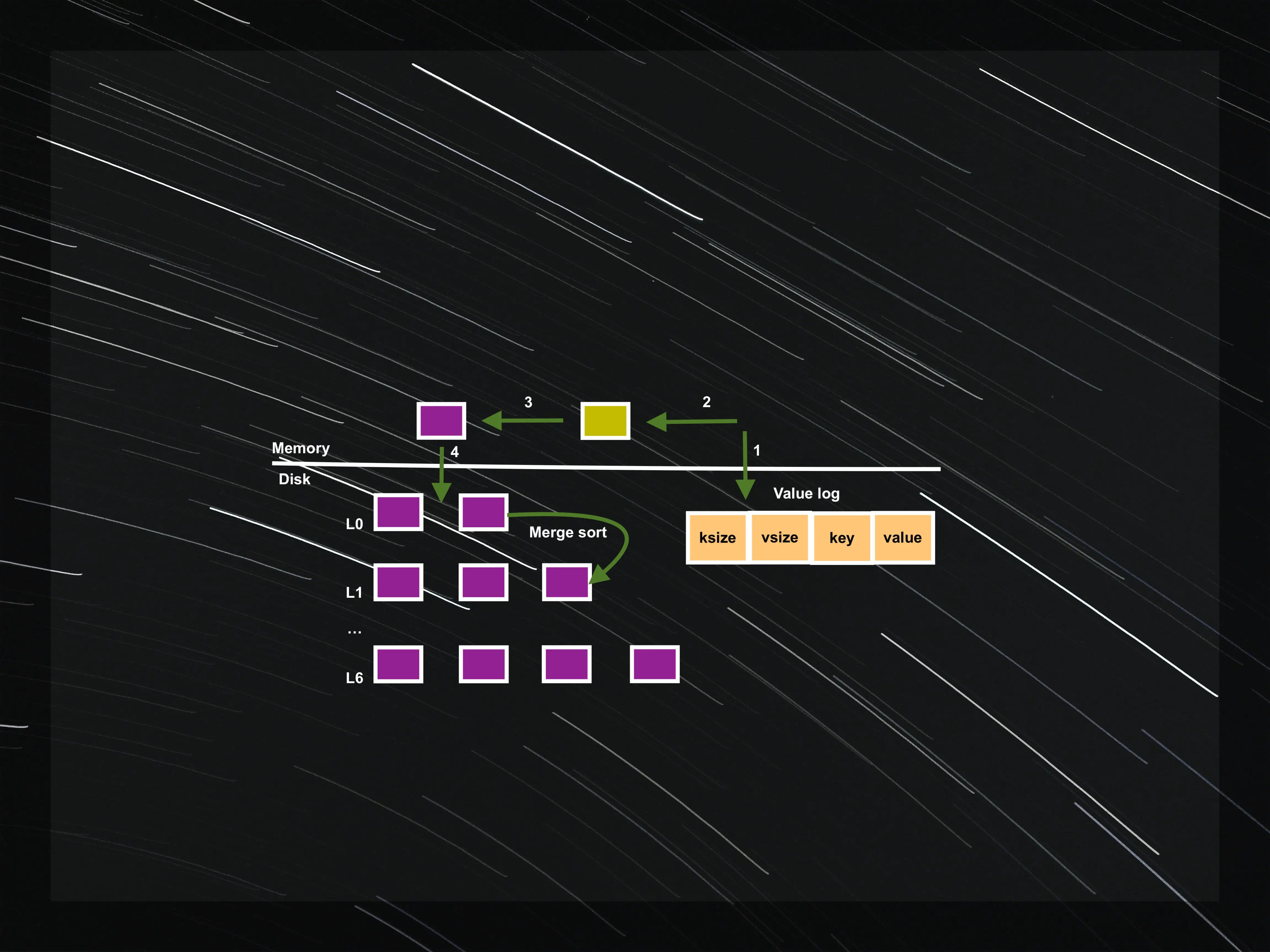
The put(key, value) operation in WiscKey modifies the original put flow. Every put(key, value) in the WiscKey adds the key-value pair in the value-log and then adds the key along with the value-log offset in the memtable. Converting the active memtable to the immutable memtable, flushing the active memtable to disk and performing the compaction process in the background remain the same.

Memtables and SSTables in WiscKey contain keys and the key-value pair offset from the value-log. Given, keys are smaller than values, the amount of data needed during compaction is significantly reduced.

Let’s look at the flow of the get(key) operation.

1. Perform get in the active memtable (RAM),
2. If not found, perform get in the immutable memtable (RAM),
3. If not found, perform get in the SSTable files.

If the get operation finds the key, a random seek to the key-value pair offset needs to be performed in the value-log to get the value. This requires an additional IO for every get operation. The research paper claims that the LSM-tree of Wisckey is a lot smaller than LevelDB, a lookup may search fewer levels of table files, and a significant portion of the LSM-tree can be easily cached in memory.

BadgerDB implements the WiscKey paper, but it makes a minor modification to put and the get operations. If the value size is less than some threshold, the value will be put in the memtable else the value-offset will be put in the memtable. If the key is found during the get operation, BadgerDB loads the value from the value-log if the retrieved value is a value-offset. SSTables always contain the value-offset.

A key in WiscKey will be deleted from the LSM-tree but the value-log remains untouched. WiscKey proposes garbage collection to remove invalid (or dangling) values from value-log.

Leverage the internal parallelism of SSDs

All the modern storage engines provide support for range queries. LevelDB provides the clients with an iterator-based interface with Seek(key), Next(), Prev(), Key() and Value() operations. To scan a range of key-value pairs, the client can first Seek(key) to the starting key, then call Next() or Prev() to search keys one by one. To retrieve the key or the value of the current iterator position, the client calls Key() or Value(), respectively.

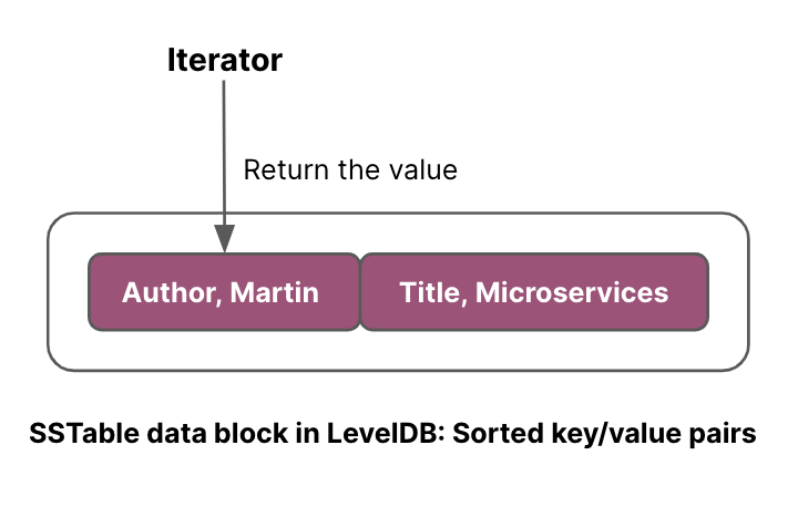
In LevelDB, since keys and values are stored together and sorted, a range query can sequentially read key-value pairs from SSTable files as shown in the image below.

However, since keys and values are stored separately in WiscKey, range queries require random reads (from value-log), and are inefficient.

Wisckey leverages the same iterator-based interface for range queries as LevelDB. To make range queries efficient, WiscKey leverages the parallel I/O characteristic of SSD devices to prefetch values from the value-log during range queries.

WiscKey tracks the access pattern of a range query. Once a contiguous sequence of key-value pairs is requested, WiscKey reads the following keys from the LSM-tree sequentially. The values corresponding to those prefetched keys are resolved in parallel (using multiple threads) from the value-log.

BadgerDB uses PrefetchSize (int) and PrefetchValues (bool) in the IteratorOptions struct [iterator.go] to decide if the values have to be prefetched. The DefaultIteratorOptions defines 100 as the prefetch size.

Introduce garbage collection

Wisckey stores only the keys in the LSM-tree and the values are managed separately. During compaction, the deleted keys will be removed from SSTable files but the values corresponding to the deleted keys will still be present in the value-log. Let’s call those values as dangling values. To deal with dangling values, WiscKey proposes a lightweight garbage collector to reclaim free space in the value-log.

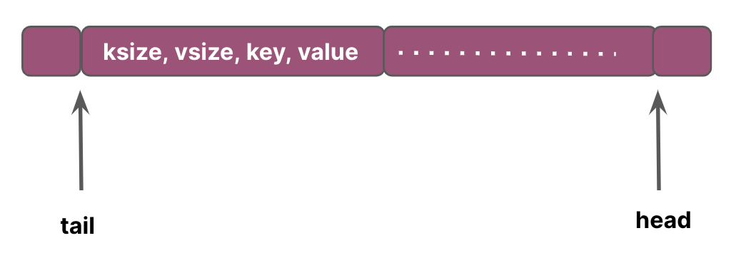
Let’s look at the structure of the value-log. Every entry in the value-log contains key-size, value-size, key and the value. The head end of this log corresponds to the end of the value-log where new values will be appended and the tail of this log is where garbage collection starts freeing space whenever it is triggered. Only the part of the value-log between the tail and the head offset contains valid values and will be searched during lookups.

Garbage collection involves the following steps:

1. WiscKey reads a chunk of key-value pairs (several MBs) from the tail offset of the value-log. It then finds which of those values are valid by querying the LSM-tree.
2. After all the valid key-value pairs are identified, the entire byte array containing the valid key-value pairs is appended to the end of the log.
3. To avoid losing any data in case a crash happens during garbage collection, WiscKey calls fsync on the value-log.
4. WiscKey needs to add the updated value’s addresses to the LSM-tree. So, it adds the key & value-offset pairs to the LSM-tree along with the current tail offset. The tail is stored in the LSM-tree as <'tail', tail-value-log-offset>.
5. Finally, the free space is reclaimed and the head offset is stored in the LSM-tree.

Quick summary

WiscKey separates values from keys in the LSM-tree. LSM-tree contains keys and the offsets of the key-value pair from the value-log. This reduces the write-amplification during compaction.
WiscKey leverages the internal parallelism offered by SSDs, during range queries.
Wisckey introduces garbage collection to remove dangling values from the value-log.

Let’s discuss various optimizations proposed in the WiscKey paper.

Optimizations offered by WiscKey

WiscKey offers two optimizations:

1. Value-Log Write Buffer: to buffer the key-value pairs before they are written to the value-log
2. Remove LSM-tree log: use value-log as recovery mechanism

Value-Log Write Buffer

For each put(key, value) operation, WiscKey needs to append the key-value pair in the value-log. Every put operation will require a write system call.

To reduce the write-overhead, WiscKey buffers the incoming key-value pairs in memory. The buffer is flushed to value-log only when the buffer size exceeds a threshold or when the user requests a synchronous insertion. This requires a change in the get operation.

Assume that a get operation finds the value-offset in the active memtable. The system needs to look up the value-offset in the value-log to get the value. With the introduction of the value-log buffer, the lookup operation will be performed in the value-log buffer first and if the value-log offset is not found in the buffer, it actually reads from the value-log.

This optimization means that the buffered data can be lost during a crash.

Removal of LSM-tree Log

The value-log is storing the entire key-value pair. If a crash happens before the keys are persistent in the LSM-tree (and after they have been written to the value-log), they can be recovered by scanning the value-log. In order to optimize the recovery of the LSM-tree from the value-log, the head offset of the value-log is periodically stored in the LSM-tree as <'head', head-value-log-offset>. When the database is opened, WiscKey starts the value-log scan from the most recent head position stored in the LSM-tree, and continues scanning until the end of the value-log. So, removing the LSM-tree log is a safe optimization.

Reference implementation of WiscKey

BadgerDB is an implementation of the WiscKey paper. We will briefly look at the put and the get implementations of BadgerDB.

Let’s start with put(key, value).

//Fields ommitted
type request struct {
	// Input values
	Entries []*Entry

	Ptrs []valuePointer
}
type Entry struct {
	Key       []byte
	Value     []byte
}
type valuePointer struct {
	Fid    uint32
	Len    uint32
	Offset uint32
}

//Code ommitted
func (db *DB) writeRequests(requests []*request) error {
	db.opt.Debugf("writeRequests called. Writing to value log")
	
	//write the requests to the value log file
	err := db.vlog.write(requests) 
	if err != nil {
		done(err)
		return err
	}
	for _, request := range requests {
		//write a single request to the LSM-tree
		if err := db.writeToLSM(request); err != nil {  
			done(err)
			return y.Wrap(err, "writeRequests")
		}
	}
	return nil
}

BadgerDB implements snapshot transaction isolation . Let’s assume the commit() method on the transaction is invoked. The commit operation results in calling the writeRequests method on db through a single goroutine in a fashion that is very much similar to a singular update queue .

As a part of this method, the key-value pairs are written to the value-log and then each request is written to the LSM-tree.

Let’s look at the writeToLSM method to understand the content of the memtable.

//Code ommitted
func (db *DB) writeToLSM(reqest *request) error {
    //Iterate through all the entries in the request
	for i, entry := range reqest.Entries {
		var err error
		if db.opt.managedTxns || entry.skipVlogAndSetThreshold(db.valueThreshold()) {
			//Write the entire key and the value in the memtable. 
			//Memtable is implemented using Skip list 
			err = db.memtable.Put(entry.Key,
				y.ValueStruct{
					Value: entry.Value,
					Meta:      entry.meta &^ bitValuePointer,
					UserMeta:  entry.UserMeta,
					ExpiresAt: entry.ExpiresAt,
				})
		} else {
			// Write the pointer to the memtable.
			err = db.memtable.Put(entry.Key,
				y.ValueStruct{
					Value:     reqest.Ptrs[i].Encode(),
					Meta:      entry.meta | bitValuePointer,
					UserMeta:  entry.UserMeta,
					ExpiresAt: entry.ExpiresAt,
				})
		}
		if err != nil {
			return y.Wrapf(err, "while writing to memTable")
		}
	}
	if db.opt.SyncWrites {
	    //Memtable contains both a WAL and a skip list. 
	    //Sync the writes to the WAL associated with the current memtable. 
		return db.memtable.SyncWAL()
	}
	return nil
}

func (e *Entry) skipVlogAndSetThreshold(threshold int64) bool {
	if e.valThreshold == 0 {
		e.valThreshold = threshold
	}
	return int64(len(e.Value)) < e.valThreshold
}

The method writeToLSM writes the entire key-value pair in the memtable if the size of the value is less than some threshold, else the encoded value of the value pointer is written to the memtable. ValuePointer references the key-value pair offset in a value-log.

Let’s look at the get(key) method.

BadgerDB maintains an array of immutable memtables to optimize reads. The get operation searches the active memtable and if the key is not found, it searches the inactive (or immutable) memtables in the reverse order (the newest immutable memtable to the oldest immutable memtable). This results in more memory pressure but to avoid GC from scanning the memory occupied by memtables, BadgerDB implements Skip list over a byte array.

//Code ommitted
type ValueStruct struct {
	Meta      byte
	UserMeta  byte
	ExpiresAt uint64
	Value     []byte
	Version uint64
}

func (txn *Txn) Get(key []byte) (item *Item, rerr error) {    
	item = new(Item)
	seek := y.KeyWithTs(key, txn.readTs)
	
	//Get the valueStruct corresponding to the key.
	//db.get will perform a get operation in all the memtables (active and all the immutable memtables), 
	//if the key is not found, it will perform a get across all the levels. 
	valueStruct, err := txn.db.get(seek)
	
	if valueStruct.Value == nil && valueStruct.Meta == 0 {
		return nil, ErrKeyNotFound
	}
	if isDeletedOrExpired(valueStruct.Meta, valueStruct.ExpiresAt) {
		return nil, ErrKeyNotFound
	}

    //if the key exists, return an item. 
    //Item will abstract the idea of fetching the value from the value-log   
	item.key = key
	item.version = valueStruct.Version
	item.meta = valueStruct.Meta
	item.userMeta = valueStruct.UserMeta
	item.vptr = y.SafeCopy(item.vptr, valueStruct.Value)
	item.txn = txn
	item.expiresAt = valueStruct.ExpiresAt
	return item, nil
}

The Get(key) method in the transaction does two things:

1. Invokes the get method of the db abstraction to get an instance of ValueStruct (represents a value)
2. If the key exists, it returns an Item. ValueStruct may or may not contain the value, so Item abstraction ensures that the value is fetched from the value-log if needed.

Let’s look at the method yieldItemValue in the Item. The idea is to decode the value pointer (get the instance of valuePointer back from the byte array) and perform a random read operation in the value-log.

//Code ommitted
func (item *Item) yieldItemValue() ([]byte, func(), error) {
	key := item.Key() // No need to copy.
	if !item.hasValue() {
		return nil, nil, nil
	}

	var vp valuePointer
	vp.Decode(item.vptr)
	
	db := item.txn.db
	//Read the value from the value log. This is a random seek in the value-log.
	result, cb, err := db.vlog.Read(vp, item.slice) 
	
	....
}

The article has already gone too long, but I would like to put a short mention of the iterator implementation in BadgerDB.

BadgerDB provides a NewIterator(opt IteratorOptions) method that returns an iterator object.

The challenge is: where should the iterator point to? Should it point to the active memtable? Or, which of the N immutable memtables or M SSTable files should it point to?

//Code ommitted
func (txn *Txn) NewIterator(opt IteratorOptions) *Iterator {
    tables, decr := txn.db.getMemTables()
    
    for i := 0; i < len(tables); i++ {
		iters = append(iters, tables[i].skiplist.NewUniIterator(opt.Reverse))
	}
	iters = append(iters, txn.db.levelController.iterators(&opt)...)
	res := &Iterator{
		txn:    txn,
		iitr:   table.NewMergeIterator(iters, opt.Reverse),
		opt:    opt,
		readTs: txn.readTs,
	}
}

BadgerDB creates iterators across all the objects: all the memtables and all the SSTable files from Level0 to the last level, and returns an instance of MergeIterator. The MergeIterator organizes all the iterators in the form of a binary tree.

//Code ommitted
type MergeIterator struct {
	left  node
	right node
}

//y.Iterator is an interface that has various implementations like skiplist.NewUniIterator, MergeIterator
func NewMergeIterator(iters []y.Iterator, reverse bool) y.Iterator {
	switch len(iters) {
    case 0:
		return nil
	case 1:
		return iters[0]
	case 2:
		mi := &MergeIterator{
			reverse: reverse,
		}
		//When we are left with 2 iterators, set the left and the right node of MergeIterator
		mi.left.setIterator(iters[0])
		mi.right.setIterator(iters[1])
		mi.small = &mi.left
		return mi
	}
	mid := len(iters) / 2
	
	//Recursive call to arrange the iterators from 0 to mid-1, and then mid to the last index
	return NewMergeIterator(
		[]y.Iterator{
			NewMergeIterator(iters[:mid], reverse),
			NewMergeIterator(iters[mid:], reverse),
		}, reverse)
}

Seek by design is a recursive operation (imagine it to be a binary tree traversal). Each iterator may find some value for the key. (The same key may be present in the active memtable and in one SSTable.) So, mi.fix() resolves the key that will be returned from the MergeIterator.

//Code ommitted
func (mi *MergeIterator) Seek(key []byte) {
	mi.left.seek(key)
	mi.right.seek(key)
	mi.fix()
}

MergerIterator is available here .

Conclusion

We have finally reached here :).

LSM-tree based storage engines typically include the following data structures:

1. On-disk log file (WAL) to persist the writes.
2. In-memory memtable(s).
3. On-disk files organized in levels.

LSM-trees offer higher write throughput because the writes are always sequential in nature, but reads are not so great because LSM-trees may have to scan multiple files or portions of multiple files. One idea to improve the reads in LSM-trees is to reduce the size of SSTable files and cache some layers of SSTables.

When designing a storage engine for SSDs, we should consider SSD characteristics including:

1. SSDs can wear out through repeated writes, the high write amplification in LSM-trees can significantly reduce the device lifetime.
2. SSDs offer a large degree of internal parallelism

The core ideas of WiscKey include: separating values from keys in the LSM-tree to reduce write amplification and leveraging the parallel IO characteristic of SSD.

I hope the article was worth your time. Feel free to share the feedback.

Mention

Thank you, Unmesh Joshi for reviewing the article and providing feedback.

References

• WiscKey
• LSM-tree
• Introducing persistent memory
• BadgerDB